Automated removal of independent components to reduce trial-by-trial variation in event-related potentials

This blogpost assumes readers are familiar with independent component analysis (ICA) in EEGLAB.

This post describes automated methods that are effective in reducing trial-by-trial variance in ERP data by removing independent components. The routines described below are written in Matlab for use with datasets saved in EEGLAB format (.set files). Sections of script are presented here: a demonstration Matlab program that applies the rejection procedures and generates graphical output can be downloaded from: http://tinyurl.com/3dvlq4k


The mixture of formal/informal style of this post is because it is based on a manuscript that was rejected for publication in a journal. The revisions requested by reviewers were too numerous for me to undertake, but, rather than just put the paper in a file drawer, I decided it would be worth describing methods here, in case others wished to try them out. I explain some of the reviewer criticisms in sections in italic, to help users evaluate the work.

UPDATE 29/10/13

Maximilien Chaumon has developed a nice EEGlab plug-in that does some of the things described here and much more! see github.com/dnacombo/autorejICA. 

Original blogpost follows:

Abstract

Background: Independent component analysis (ICA) is a method for decomposing an EEG signal into temporally independent sources. Only some of the independent components (ICs) will reflect cortical activity that relates to cognitive processing relevant to a task of interest.
Method: Algorithms were developed for removing ICs that are (a) noisy; (b) highly focal; (c) highly spatially asymmetric; (d) have low signal-to-noise ratio, or (e) show high trial-by-trial variability. Their impact was evaluated using auditory event-related data from 10 adults and 10 children.
Results: Removal of ICs identified by algorithms (a)-(e) had little impact on the averaged waveforms, but reliably reduced trial-by-trial variance of peaks of interset and increased inter-trial phase coherence.
Conclusions: The algorithms can improve reliability of measurement of event-related potentials, as well as focusing attention on ICs that reflect meaningful event-related brain activity.

Introduction

The electroencelphalogram (EEG) recorded from electrodes placed on the scalp can provide information about underlying brain activity, but attempts to interpret the recorded signal are invariably hindered by the presence of artefact, i.e. electrical signals that are unrelated to event-related brain activity. These may come from non-brain sources such as eye and muscle movements, as well as poorly attached electrodes or line noise. In event-related studies, the EEG recording is divided into trials locked to a marker that denotes a specific stimulus or response. A common method for reducing the impact of artefact is to discard trials where the amplitude on any channel exceeds some absolute threshold, such as ± 75 microvolts. Recently, more sophisticated procedures for artefact rejection have been developed, based on higher-order statistics (Delorme, Sejnowski, & Makeig, 2007). These methods are useful for detecting portions of the EEG signal that contain unsystematic artefacts, such as those caused by large body movements.

Some artefacts, however, have a more stereotyped morphology and recur in the signal. Eyeblinks are the most obvious large artefact of this kind. Although the impact of eyeblinks can be removed by discarding trials in which they are detected, this is less efficient than adopting a procedure that identifies their presence in the data and corrects for it. Semlitsch, Anderer, Schuster and Presslich (1986) developed a regression-based approach to ocular artefact reduction which is implemented in Neuroscan© software and is widely used. Jung et al (2001) adopted a different approach based on independent component analysis (ICA). This involves decomposing the EEG into a mixture of signals with temporally independent sources, some of which correspond to unwanted noise, such as eyeblinks, muscle artefact or heartbeat (Onton, Westerfield, Townsend, & Makeig, 2006). However, although plots of the independent component (IC) activations and their sources make a compelling case for the usefulness of this approach in separating difference sources of the scalp signal, it is usually left to the investigator to scrutinise the ICA output and judge which components are artefacts. This has three disadvantages over automated procedures: first, it is subjective and therefore not fully replicable; second, it makes it possible to bias results of a study by selection of specific components; and third it is time-consuming, given that there are usually as many ICs as there are recording channels for each participant. To address this issue, Campos Viola, Thorne, Edmonds, Schneider, Eichele, and Debener (2009) developed a semi-automatic method for identifying ICs corresponding to EEG artefact. Their method involves matching templates for IC activations across participants, so that those that have common features, such as predominant activity in eye channels, can be identified. This approach, however, would not be useful in cases where there is idiosyncratic artefact that does not generalise across participants.

The goal of the current paper is to take the approach of Jung et al (1998, 2001) one step further, and automate the detection and removal of artefactual components. This approach grew from an initial method used by Bishop and Hardiman (2010), who removed components that were unlikely to reflect event-related activity because they had high trial-by-trial variance. Subsequently, Bishop, Hardiman and Barry (2011) used a different automated approach, in which artefactual components were identified as those with highly focal sources. In the current paper, experimental datasets are used to explore the impact of these and other methods for identifying and removing artefactual components.

Reviewers pointed me to three recent papers of which I’d been unaware, which offer alternative approaches to automated IC removal. They suggested I do an explicit comparison of my methods with these, and with subjective evaluation by experts. A good idea, but I can't justify the time, given my other committments. But could make a nice student project for someone?
Mognon, A., Jovicich, J., Bruzzone, L., & Buiatti, M. (2011). ADJUST: An automatic EEG artifact detector based on the joint use of spatial and temporal features. Psychophysiology, 48(2), 229-240. doi: 10.1111/j.1469-8986.2010.01061.x
Nolan, H., Whelan, R., & Reilly, R. B. (2010). FASTER: Fully Automated Statistical Thresholding for EEG artifact Rejection. Journal of Neuroscience Methods, 192(1), 152-162. doi: 10.1016/j.jneumeth.2010.07.015
Wessel, J. R., & Ullsperger, M. (2011). Selection of independent components representing event-related brain potentials: A data-driven approach for greater objectivity. Neuroimage, 54(3), 2105-2115. doi: 10.1016/j.neuroimage.2010.10.033

Methods

Datasets
The artefact removal algorithms are demonstrated using a subset of data from an auditory ERP paradigm, previously reported by Bishop, Hardiman, and Barry (2011). Data from 10 children and 10 adults were selected from consecutive series of data files of typically developing children and parents.

The stimuli were pure tones of duration 175 ms, windowed at 15 ms, presented monaurally to the right ear at 86.5 dB SPL through sound attenuating Sennheiser HD25-1 headphones. There were 666 tone stimuli, including sinusoids of frequency 1000 Hz (70% trials), 1200 Hz (15% trials) or 1030 Hz (15% trials), presented in a quasi random sequence with stimulus onset asynchrony of 1 s. All stimuli were treated together for ICA.

Participants were seated in a sound-attenuated electrically-shielded booth, and played Gameboy, or watched a silent DVD or video during stimulus presentation.

The EEG was recorded on a SynAmps or NuAmps NeuroScan Inc. system. An electrode cap was fitted to record from sites: FC1, F7, FP1, Fz, FP2, F8, FC2, FT9, FC5, F3, FCz, F4, FC6, FT10, T7, C3, Cz, C4, T8, CP5, P7, P3, Pz, P4, P8, CP6, M1, and M2. One mastoid was used as reference electrode and ground was placed at AFz. Electro-oculograms were recorded from supra- and infra-orbital electrodes on the left eye and also from electrodes placed lateral to the left and right eyes. The continuous EEG was digitised at 500 Hz and band-pass filtered (0.01 – 70 Hz for SynAmps; 0.1 – 70 Hz for NuAmps) and a 50 Hz notch filter was employed.

EEGLAB open source software (Delorme & Makeig, 2004) was used for all subsequent processing steps. The bipolar electro-oculograms were subtracted to give vertical (VEOG) and horizontal (HEOG) eye movement channels. Raw EEG data were downsampled to 250 Hz, high pass filtered at 0.5 Hz, re-referenced to the mean mastoids, and divided into 1000 ms trials including a baseline of 200 ms.

Data processing

1. Rejection of noisy epochs

Onton et al (2006) emphasise that we need to distinguish between two kinds of artefact, namely, (a) the unsystematic noise that affects a signal when, for instance, a participant makes a large movement, and (b) the more systematic noise that is generated by specific physiological phenomena, such as blinks, heart beat, or regular muscle movements. ICA is useful for identifying and removing only the latter kind of artefact, and so it is necessary first to use more conventional methods to remove trials containing unsystematic noise. This was done using the automated artefact rejection routine from EEGLAB, which is described by Delorme, Sejnowski, and Makeig (2007). The eye channels were excluded from this processing, because it is not desirable to lose trials that contain systematic artefact that can be corrected for. This line of the Matlab program achieves this, after defining an array, inchan, containing the number of the channels that are included in artefact rejection (e.g., inchan = 1:28)

[EEG, rmepochs] = pop_autorej( EEG, 'electrodes', inchan);

(The AUTOICREJ program also offers the option of more conventional artefact rejection by removal of trials where the amplitude exceeds a specified threshold).

2. Independent component analysis

EEGLAB offers a variety of options for performing ICA. I've found second order blind identification (SOBI) a good method in terms of speed and results (see Delorme et al, unpublished for comparison of methods).
This was applied, with the following command:

EEG = pop_runica(EEG, 'icatype', 'sobi', 'dataset',1, 'options',{});


3. Identification of independent components for removal

Five methods were used to identify ICs for removal, as follows:

(a) Noisy components. Some components have activations that do not correspond to a smooth waveform, but rather resemble random noise. These components can be identified by considering the autocorrelation of values of the ICA activation over time. In a smooth waveform, each datapoint will be highly predictable from the few preceding datapoints. In a noisy waveform, this is not the case. One needs to set an arbitrary cutoff to identify unacceptably noisy components. The default in AUTOICREJ is autocorrelation below .5 for points separated by 12 ms is taken to indicate a noisy component.

The section of script achieving this criterion is as follows:

%----------------------------------------------------------------
% Identifying noisy components
%----------------------------------------------------------------
ncomp= length(EEG.icawinv); % ncomp is number of components
dropautocorr=.5; % Will drop components with autocorrelation less than this value;
mycorrint=round(12/(1000/EEG.srate)); %  find N pts corresponding to 12 ms
for k=1:ncomp
 rej(k)=0; % initialise
 y=squeeze(EEG.icaact(k,:,:));
 yy=xcorr(mean(y'),mycorrint,'coeff'); %autocorrel for pts sep by 12 ms
 if yy(1)< dropautocorr
  rej(k)=1; % codes reject/accept for this component
 end
end
%----------------------------------------------------------------


To see which components are selected for removal, inspect the rej vector; this will have values of 1 for those components identified for rejection by this routine. Figure 1 shows mean activations for the first 15 ICs for a demonstration case. ICs 5 and 9 were selected for removal by this routine.

Figure 1: Mean activation for ICs 1-15 in demonstration case

Neither reviewer raised any difficulties about this routine. As can be seen in the examples in Supplementary Figures, it identifies components that are easy to pick out by eye as being noisy.

(b) Components arising from a focal source. Components that correspond predominantly to the activity at a single channel are likely to be noise. Bishop et al (2011) proposed an easy way to identify such focal activity by using the standardized inverse weight matrix from the ICA decomposition, excluding components which have an absolute z-score above a critical value. The critical value may need to be determined by trial and error. Because blinks typically have virtually all their activity on the vertical EOG channel, our experience is that a z-score cutoff of 4 will usually identify them datasets with small electrode arrays. That is the default cutoff used in AUTOICREJ.

The code for this rejection routine is as follows:

%----------------------------------------------------------------
% Find components with focal activity
%----------------------------------------------------------------
ncomp= length(EEG.icawinv); % ncomp is number of components
focalICAout = 4; % default zscore cutoff
c=zscore(reshape(EEG.icawinv,1,ncomp*ncomp));
b=reshape(c,ncomp,ncomp); %making zscores in relation to whole matrix of winv
%creates standardized winv matrix with channels as row and components as cols
for k=1:ncomp
 rej(k)=0; % initialise
 mywt=sort(abs(b(:,k)),'descend'); %sorts standardized weights in descending order
 if mywt(1) > focalICAout %corrected 11/9/11
 end
end
%----------------------------------------------------------------

Figure 2 shows the headplots for ICs for the same participant as Figure 1.The headplots map the relative projection weights at each electrode to a given IC.  Components 1, 2 and 4 are selected for rejection by this routine.



Figure 2: Topography of inverse weights for components 1-15

One of the referees was sceptical about the trial-and-error rationale for determining a z-score cutoff “because one would have to find a threshold potentially for every scalp montage or even subject”. Certainly, if thresholds were set separately for each participant, this would defeat the object of the exercise, and that is not what is recommended. My experience is that one needs to look at the outputs of an initial set of data to check how well a cutoff identifies components that have the appearance of blinks, but once a cutoff is selected, it should be applied to the whole dataset for a given paradigm. With a stringent cutoff, the most common ‘error’ here is to fail to reject a blink component, rather than to erroneously categorise a biological component as artefact, but true artefacts will usually be picked up by one of the other routines, if they are missed by this one.

The reviewer also suggested “there are better ways of classifying outliers than simple z-scores (for which the datapoints in the weights matrix would also have to be normally distributed, which is not always the case).” I disagree; you don't need a normally-distributed set of weights to use this criterion. A z-score of 4 corresponds to a probability of around 1 in 30,000, and so will not occur in a small weight matrix (i.e. with 64 channels or less) unless the weights distribution is strongly skewed.

The reviewer is right to point out that we can't assume that this z-score value would work with other montages. A more extreme cutoff may be required if applying the criterion to large electrode arrays.

(c) Highly asymmetrical components. Brain generators of responses to auditory signals are usually symmetrical. Symmetry of the underlying generator of a component can be quantified by comparing the inverse weight matrix for left-sided channels with corresponding right-sided channels. This is a 2 dimensional matrix of values, where rows correspond to channels, and columns correspond to components. The values in the matrix reflect the strength of the loading of a channel on a component. The whole matrix is first transformed to z-scores. For each component and each channel pairing, a value is computed corresponding to the absolute difference between the left and right channel standardized inverse weights. The maximal difference is taken as an index of asymmetry. As with the other routines, the cutoffs for dropping components are initially selected by trial and error after scrutinising the data. In AUTOICREJ the default value is 3.5z.

%----------------------------------------------------------------
% Find asymmetric components
%----------------------------------------------------------------
mycriterion=3.5; % criterion for z-score difference between paired L-R electrodes
w=zscore(EEG.icawinv); %inverse wt matrix created when ICA is run
nelec=EEG.nbchan;
ncomp= length(EEG.icawinv); % ncomp is number of components
for k=1:ncomp
 rejindex(k)=0;
 rej(k)=0;
 alldiff=[]; %initialise array to hold difference values for this component
 for myelec=1:nelec % check all electrodes to find L-R pairs
  mylab=EEG.chanlocs(myelec).labels;
  seekelec='';
  mynum=str2num(mylab(length(mylab))); % take last character of channel name
  if (mod(mynum,2)==0); %find channel with even number
   seekelec=strcat(mylab(1:length(mylab)-1),num2str(mynum-1));
%seekelec is channel label for corresponding odd channel
  end
 if length(seekelec) > 0
   matchelec=0; %initialise matchelec
   for thiselec=1:nelec
    if strcmp(EEG.chanlocs(thiselec).labels,seekelec)==1
    matchelec=thiselec; %channel number for corresponding odd
   end
  end
 if matchelec > 0
   latdiff=abs(w(myelec,k)-w(matchelec,k));
   %latdiff is difference in inverse weights for corresponding L and R electrodes
   alldiff=[alldiff latdiff]; %save in array of paired differences for this component
   end
   rejindex(k)=max(alldiff); % save max value across all electrode pairs
  end
 end
end
for k=1:ncomp
 if rejindex(k) > mycriterion
 rej(k)=1;
 end
end
%----------------------------------------------------------------


For the dataset in Figures 1 and 2, this routine identifies ICs 3, 9 and 11 for rejection.

In AUTOICREJ, the method for identifying asymmetrical components has been extended to identify components corresponding to eye movements and blinks. To do this, the vertical and horizontal eye movement channels are treated as a pair, with inverse weights for these two channels being subtracted for each component. Where the component has high activity on either channel, this will give a high asymmetry score. (As noted below, with this method implemented, it was not necessary to include step (b), focal components, to identify blinks, as the same ICs were selected by both methods).

The reviewers were particularly critical of this routine, on two counts.
i) They pointed out that researchers might be particularly interested in asymmetric generators, e.g. lateralized frontal activity on stopping paradigms, or motor activity in uni-manual tasks. I had already anticipated this point and noted that you might not want to use this rejection method in all paradigms; I have, however, found it useful for auditory ERPs, where symmetric generators are expected.
ii) There was concern that minor shifts in cap position and / or brain anatomy between subjects might lead to symmetrical brain sources being not perfectly represented on the scalp level; “this is particularly true for denser electrode arrays than the ones used by the author. In a high density array, from my understanding, this method is particularly likely to be inaccurate if a symmetric component is not perfectly symmetric on the sensor level, leading to a (even slightly) contorted IC map representation.” I think it is unlikely that this kind of asymmetry would trigger rejection by this condition. First, the asymmetry needs to be substantial to meet the cutoff of 3.5z. Second, a z-score difference this large is unlikely to be met unless the asymmetry is based on a single electrode pair. If asymmetric activity is spread over a range of electrodes, z-scores differences won't be high enough to generate a big difference in any electrode pair. In effect, you need an outlier just on one side, rather than a patch of activation across adjacent electrodes. Having said that, I'd be very interested to see this method evaluated with large montages.

(d) Components with low signal-to-noise ratio (SNR). This method evaluates components in terms of their relationship to time-locked events. It simply measures the ratio of activity in the baseline period to activity in a post-baseline period of interest (POI), and rejects components where the SNR falls below a pre-specified cutoff. In this section of script the POI is specified as 0 to 500 ms post-onset:
%----------------------------------------------------------------

% Find components that have SNR greater than threshold
%----------------------------------------------------------------
%NB need to specify epochpt1 and epochpt2 to focus on period of interest (POI)
SNRcut=1.3; % default value for cutoff on ratio of SD post/pre baseline
startPOI=0;
endPOI=.5; %end of period of interest in seconds
epochpt1=(abs(EEG.xmin)+startPOI)*EEG.srate; %data pt for start of POI
epochpt2=(abs(EEG.xmin)+endPOI)*EEG.srate; %data pt for 3ne or POI
zz=zscore(EEG.icaact);
for k=1:ncomp
 rej(k)=0;
 av1=mean(zz(k,epochpt1:epochpt2,:),3);%activity in POI
 av2=mean(zz(k,1:epochpt1,:),3); %activity in baseline
 thisrej=std(av1)/std(av2); %SNR comparing trial with baseline
 if thisrej < SNRcut
  rej(k)=1;
 end
end
%----------------------------------------------------------------

This routine identified components, 2, 3, 5, 8 and 9 for rejection (see Figure 1).

One reviewer raised several queries:
a) How to select a cutoff. Again, this is arbitrary. ICA activations are converted to z-scores to give a common scale; the default value of 1.3 was obtained by trial and error.
b) Some of the components identified this way look event-related. This may be so, but their removal makes very little difference to the averaged waveform, because they are either small or noisy. This is probably more of an issue for researchers who are interested in identifying and localising independent signal sources, even if they are small. But for those who plan to analyse features of the averaged waveform after component removal, this is less of an issue, because removal of components with such small contribution to activity has little effect.
c) What happens if a component represents an event-related potential occurring before an event? The answer is that if you are using a paradigm where anticipatory responses are of interest, you would need to respecify the time windows for measurement of the signal to noise ratio. The AUTOICREJ program assumes the baseline is the comparison interval, but it need not be. The key values are av1 and av2, which by default are computed from epochpt1:epochpt2 (POI) and 1:epochpt1 (baseline).

(e) Components with high trial-by-trial variance. This was based on the original method used by Bishop and Hardiman (2010). Like routine (d), it evaluates components in terms of their relationship to time-locked events. The logic is that if we are interested event-related activity, we expect to see a consistent relationship between the event and the component activation from one trial to the next. Artefacts are unlikely to be synchronised with events, and so they will show high trial-by-trial variance.

%----------------------------------------------------------------
% Find components that have trial by trial variability greater than average
%----------------------------------------------------------------
ncomp= length(EEG.icawinv); % ncomp is number of components
zz=zscore(EEG.icaact);
for k=1:ncomp
 B=zz(k,epochpt1:epochpt2,:); % epochpt1 and 2 defined in previous routine for POI
 meanabs=squeeze(mean(sqrt(B.*B))); %mean absolute for each trial
 rejindex(k)=std(meanabs); %will be high if there is high trial-to-trial variation
end
stdlist=rejindex;
m=mean(stdlist); % stdlist is vector of stdev values for all components
st=std(stdlist);
crit=m+st; % criterion here is trial-by-trial std in top 16% of values for components
 for k=1:ncomp
  if rejindex(k) > crit;
  rej(k)=1;
 end
end
%----------------------------------------------------------------


This method selected components 1 and 2 for removal for the dataset shown in Figures 1 and 2. These are components already identified by other criteria as blinks.

As discussed below, however, for the dataset as a whole, this method seemed the least satisfactory, sometimes identifying components for rejection that looked biologically plausible. This may have been because this is the only routine that picks components on the basis of their properties relative to other components. In other words, it will always select a proportion of components (those with variability greater than 1 SD above the mean, i.e. usually around 16%) regardless of the absolute level of the signal. Thus  all participants will have a similar proportion of ICs selected by this method. It’s possible that it would work better if an absolute cutoff was used. However, Bishop and Hardiman (2010) adopted this approach, but they did have difficulty specifying a single cutoff that was effective for all participants.
4. Removal of artefactual components. This was achieved by EEGLAB’s pop_subcomp routine.  AUTOICREJ keeps a tally of which ICs meet the five criteria for rejection, and displays the headmaps and mean activation timecourse for each component together with code letters that indicate which rejection criteria were met. This allows the user to check how far the routines identify components that agree with a selection based on visual inspection.

5. Assessing impact of the component removal. This was done by inspecting the grand averaged waveform to standard tones across all epochs. In addition, the trial-by-trial variability of the P1 and N1 peaks was computed for each participant, as well as inter-trial coherence (ITC), which is a measure of the extent to which oscillations at a given frequency are in phase from trial to trial. For the auditory ERP data considered here, we expect high ITC in an interval from around 0-300 ms post stimulus onset in the delta, theta and alpha frequency bands (cf. Bishop, Anderson, Reid, & Fox, 2011).

Results

Detailed results for a demonstration dataset (Adult #02) are presented for illustrative purposes; full results for the remainder of the sample are available from the Oxford University Research Archive . The full script for AUTOICREJ is also available from that site.

Figures 3 and 4 show IC maps and corresponding activation plots for participant Adult #02; components that met one or more criteria for removal are labelled in red, with letters denoting which criteria were met.




Figure 3 Headplots and back-projected activation traces (activation by time in ms) for independent components 1-15 for participant Adult #02

ICs identified by artefact algorithms are shown in red, with the criterion for rejection given below IC number. Polarity of activation is arbitrary. For instance, IC2 shows focal activity on the VEOG channel, indicative of blinks, and is rejected on the criteria of asymmetry (A), focal activity (F), and high trial-by-trial variance (V). IC4 has a head-plot indicating symmetrical fronto-central activity, characteristic of a biologically plausible component, but is rejected because activity in the baseline means it has a low signal-noise ratio (S). IC7 is rejected because of asymmetric (A), focal (F) activity plus a noisy activation trace (N). Overall, eleven of the 28 ICs for this participant were retained, and for most of these the averaged activation plot shows phasic activity in the first 200 ms of the post-baseline period.



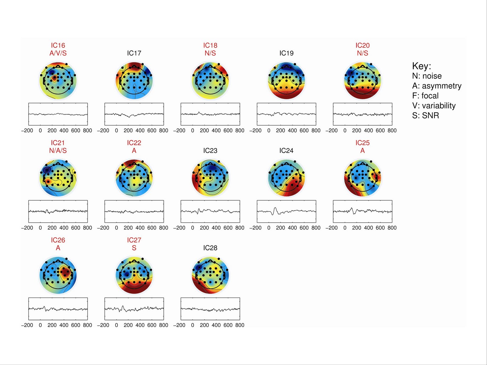Figure 4; as for Figure 3, Components 16-28

For the sample as a whole, there was wide variation in the number of accepted ICs: for adults the mean was 6.9, range 2 to 11; for children the mean was 10.7, range 2 to 15. Thus in general, only 20-40% of ICs were retained.

One referee suggested that the if only two ICs are retained, this suggests the quality of the data was poor. But if you look at the data for participants with few retained components (see Adult #07 in supplementary material), the auditory ERP looks clean, and it is barely affected by dropping all but two ICs.

Scrutiny of the rejection status of ICs for all 20 participants confirmed that the criterion (b), focal activity, was redundant; because the program was set to treat VEOG and HEOG electrodes as a pair, focal activity was almost always identified by the asymmetry criterion, and in the few cases where it was not, it co-occurred with noisy activation or low SNR. This criterion could therefore be disregarded. However, it is recommended that this criterion be used if criterion (c), asymmetric activity, is dropped. As can be seen from the data in Supplementary Material, it is effective in detecting blinks.

In addition, it was decided also to exclude the criterion of high trial-by-trial variance, as this sometimes led to exclusion of ICs that appeared biologically plausible, especially in children’s data - see e.g., Child #06, IC4.

The figures in Supplementary material also show the average auditory ERP for individual participants, for (i) original data; (ii) after artefact rejection; and (iii) after removing components identified because of noisy data, asymmetry or low SNR (with this step being conducted on the results of step ii).

It is evident from inspection that the waveform shape is generally preserved after component removal. Mean amplitudes at Fz for time windows corresponding to P1 and N1 (children: P1 = 44-104 ms, N1 = 108 to 188 ms; adults, P1 = 40-72 ms; N1= 76-140 ms) are shown in Table 1.




Table 1

Mean (SD) statistics for averaged ERPs in the P1-N1 interval, according to method of artefact rejection

For each peak the means were compared using repeated measures ANOVA for the three rejection conditions and two age bands. The Greenhouse-Geisser correction for violations of sphericity was applied. There was no significant effect of rejection condition, F (1.18, 36) = 2.25, p = .12, indicating that the size of these mean amplitudes was unaffected by either rejection of artefactual trials, or removal of artefactual ICs. However, trial-by-trial variance of peaks was significantly affected by removal of artefactual ICs, F (1.07, 19.3) = 38.4, p < .001, partial eta squared = .68. As can be seen from the individual data in Supplementary material, traditional artefact rejection reduced trial-by-trial variance in all participants; subsequent IC removal further reduced this variation in all but one participant (Child #06).
A related measure of trial-by-trial stability is the phase-locking measure of ITC. Peak ITC in the time window of 0 to 300 ms was computed for each participant in each artefact rejection condition. The means, shown in Table 1, were subjected to repeated measures ANOVA, which indicated a significant effect of artefact removal method, F (1.21, 21.83) = 10.67, p = .002, partial eta squared = .37. Post hoc tests indicated that there was no difference in ITC for the uncorrected data and traditional artefact rejection, but the peak ITC was substantially larger for the IC removal method than for traditional artefact rejection, F (1, 18) = 10.87, p = .004, partial eta squared = .38.

Discussion

ICA decomposes EEG signals into biologically meaningful elements, but to date selection and interpretation of ICs has been a largely subjective process. The automated routines described here can be used to select those components that have a plausible distribution of activity, both in space and time, while excluding the activity of ICs that appear to arise from non-brain physiological processes, or which are unrelated to events of interest. Activity of these components can be removed with little impact on indices such as ERP peaks. The benefit of removing artefactual components is that it reduces trial-by-trial variability in signal amplitude, giving a more reliable measure, and providing stronger evidence of event-related phase-locking.

The usefulness of these artefact rejection routines may vary according to the experimental paradigm. For instance, in studies concerned with motor responses or somatosensory recordings, there might be specific interest in asymmetric activity, such as is seen with mu-rhythm. In such a case, the algorithm for focal activation could be used instead of the asymmetry algorithm. Overall, it must be emphasised that automated artefact rejection is unlikely ever to supersede human judgement completely; it is important to evaluate the output rather than unthinkingly apply artefact rejection procedures. Nevertheless, the algorithms presented here can facilitate data reduction, making it easier for researchers to focus on ICs that are relevant to a specific experimental paradigm, and to identify clusters of similar ICs across participants.

References

Bishop, D. V. M., Anderson, M., Reid, C., & Fox, A. M. (2011). Auditory development between 7 and 11 years: An event-related potential (ERP) study. PLoS One, 6(5),
e18993. doi: 10.1371/journal.pone.0018993

Bishop, D. V. M., & Hardiman, M. J. (2010). Measurement of mismatch negativity in individuals: a study using single-trial analysis. Psychophysiology, 47, 697-705

Bishop, D. V. M., Hardiman, M. J., & Barry, J. G. (2011). Is auditory discrimination mature by middle childhood? A study using time-frequency analysis of mismatch responses from 7 years to adulthood. Developmental Science, 14, 402-416.

Campos Viola, F., Thorne, J., Edmonds, B., Schneider, T., Eichele, T., & Debener, S. (2009). Semi-automatic identification of independent components representing EEG artifact. Clinical Neurophysiology, 120(5), 868-877.

Delorme, A., & Makeig, S. (2004). EEGLAB: an open source toolbox for analysis of single-trial EEG dynamics including independent component analysis (sccn.ucsd.edu/eeglab/). Journal of Neuroscience Methods, 134, 9-21.

Delorme, A., Sejnowski, T., & Makeig, S. (2007). Enhanced detection of artifacts in EEG data using higher-order statistics and independent component analysis. Neuroimage, 34(4), 1443-1449.

Jung, T.-P., Makeig, S., Westerfield, M., Townsend, J., Courchesne, E., & Terrence J. Sejnowski. (2001). Analysis and visualization of single-trial event-related potentials. Human Brain Mapping, 14(3), 166-185.

Onton, J., Westerfield, M., Townsend, J., & Makeig, S. (2006). Imaging human EEG dynamics using independent component analysis. Neuroscience and Biobehavioral Reviews, 30, 808-822.

Semlitsch, H. V., Anderer, P., Schuster, P., & Presslich, O. (1986). A solution for reliable and valid reduction of ocular artefacts, applied to the P300 ERP. Psychophysiology, 23, 695-703.